How to Value a Gold Mine: NAV and DCF Walkthrough

NAV for screening, DCF for detail

Net Asset Value (NAV) and discounted cash flow (DCF) are the standard approaches for operating and development-stage mines. NAV standardises price, discount rate, and mine life so you can rank peers quickly; DCF models year-by-year production and costs when you need asset-specific schedules.

The worked examples below use the same fictional mine for both methods.

Understanding Reserve-Based NAV

The NAV Framework

Net Asset Value (NAV) is calculated by summing the present value of all ore reserves at standard assumptions:

NAV = PV(revenue from reserves) − PV(capital costs) − PV(operating costs) − PV(taxes and royalties)

Reserves means proven and probable: the ore that has been drilled out and shown to be economic to mine. It is the smaller, harder number. Resources are everything else the geologists think is down there, and a mine life built on resources rather than reserves is a promotional document.

NAV expresses value per share by taking the discounted value of the assets, deducting net debt to get to equity, and dividing by diluted shares outstanding. Forgetting the net debt step is the common error, and on a geared miner it flatters the answer by the whole borrowing.

Standard NAV Assumptions

Most institutional investors use these baseline assumptions for NAV calculations:

• Gold Price: Forward curve for the first 2-3 years, then a flat long-term assumption reflecting your view of marginal cost of production. The worked examples below use $3,500/oz.
• Discount Rate: 5–8% for Tier-1 jurisdictions (Canada, Australia), 8–12% for emerging markets. See mining discount rates by jurisdiction for detailed guidance.
• Mine Life: Based on proven and probable reserves only, often 10–20 years
• AISC: Company guidance, adjusted for inflation
• Tax Rate: Jurisdictional statutory rate (30–35% in most countries)

The advantage of NAV is that it produces apples-to-apples peer comparisons. A gold company trading at $20/share against a modelled NAV of $35/share sits at about 0.57× NAV under those assumptions.

A Worked NAV Example

Consider Company X, an operating gold mine:

Reserves: 4.75 million ounces of contained gold, proven and probable Annual Production: 500,000 oz/year for the first six years, tapering to 400,000 oz by Year 10 as grades fall (10-year mine life) AISC: $1,500/oz at plateau (all-in sustaining cost, which already includes sustaining capital, corporate G&A, and reclamation), rising in the later years Tax Rate: 30% (including all royalties and government levies) Gold Price Assumption: $3,500/oz Discount Rate: 7%, a Tier-1 operating mine

A mine’s cash flows are not flat, so the NAV is built year by year. Grades decline as the pit deepens: the ounces come slower, and each one costs more, because the operation’s fixed costs spread over fewer ounces and the haul from the pit floor gets longer. Company X holds 500,000 oz/year through Year 6, then tapers to 400,000 oz by Year 10 with AISC drifting from $1,500/oz to $1,700/oz.

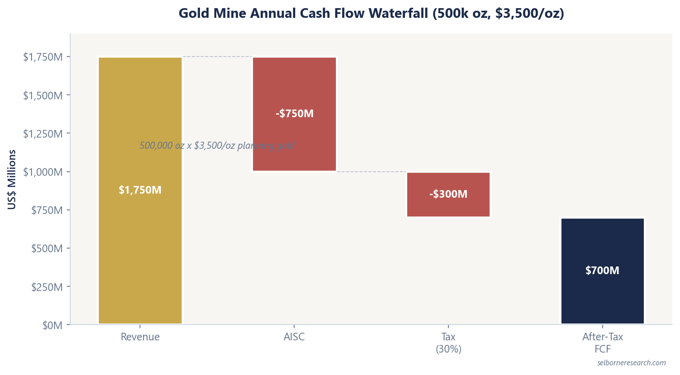
Annual free cash flow in the plateau years (1-6):

• Revenue: 500,000 oz × $3,500 = $1,750 million
• AISC: 500,000 oz × $1,500 = $750 million
• Pre-tax FCF: $1,000 million
• Taxes (30%): $300 million
• After-tax FCF: $700 million

Note that AISC is the cost line, not cash operating costs. Since AISC already includes sustaining capex, there is no separate capital deduction. If you use cash costs instead (say $1,100/oz), you must subtract sustaining capex separately. Mixing the two is a common modelling error that double-counts capital.

The year-by-year build, discounted at 7%:

Year	Oz Prod	Gold Price	Revenue	AISC/oz	AISC Cost	Tax (30%)	After-Tax FCF	Discount Factor	PV
1	500k	$3,500	$1,750.0M	$1,500	$750.0M	$300.0M	$700.0M	0.935	$654.5M
2	500k	$3,500	$1,750.0M	$1,500	$750.0M	$300.0M	$700.0M	0.873	$611.1M
3	500k	$3,500	$1,750.0M	$1,500	$750.0M	$300.0M	$700.0M	0.816	$571.2M
4	500k	$3,500	$1,750.0M	$1,500	$750.0M	$300.0M	$700.0M	0.763	$534.1M
5	500k	$3,500	$1,750.0M	$1,500	$750.0M	$300.0M	$700.0M	0.713	$499.1M
6	500k	$3,500	$1,750.0M	$1,500	$750.0M	$300.0M	$700.0M	0.666	$466.2M
7	480k	$3,500	$1,680.0M	$1,550	$744.0M	$280.8M	$655.2M	0.623	$408.2M
8	450k	$3,500	$1,575.0M	$1,600	$720.0M	$256.5M	$598.5M	0.582	$348.3M
9	420k	$3,500	$1,470.0M	$1,650	$693.0M	$233.1M	$543.9M	0.544	$295.9M
10	400k	$3,500	$1,400.0M	$1,700	$680.0M	$216.0M	$504.0M	0.508	$256.0M

Total production is the full 4.75 Moz reserve. Summing the PV column gives an asset NAV of $4,645 million.

The back years earn less and are discounted harder, so they add little: Year 10 produces 80% of Year 1’s ounces but only 39% of its present value. That is the shape a flat average hides.

Add residual value (salvage of land and infrastructure at Year 10):

• Assume 10% of Year-1 FCF = $70 million
• PV = $70M × 0.508 (Year-10 discount factor) = $35.6 million

Total asset value: $4,645M + $35.6M = $4,680 million

Less: Net Debt (assume $150 million net debt):

• Equity Value: $4,680M - $150M = $4,530 million

Shares Outstanding: 100 million (fully diluted)

NAV per Share: $4,530M / 100M = $45.30/share

A flat annuity is the quick screening shortcut: $700M × 7.02 (the 10-year annuity factor at 7%) gives roughly $4,914M. That runs about 6% above the year-by-year answer because it assumes every year looks like Year 1. Use it to rank a screen, never to set a target.

Company X trading at $25.00/share would sit at about 0.55× the $45.30 modelled NAV under those assumptions. Substitute a different long-term gold assumption and re-run; NAV is highly sensitive to the commodity price input.

Discounted Cash Flow (DCF) Valuation

When to Use DCF Over NAV

DCF is preferred when:

• Mine life is short (5–7 years) and residual value matters
• Commodity prices need stress-testing rather than a single flat assumption
• Several mines or projects carry different risk profiles
• Cost inflation or capex schedules vary materially year by year

NAV is preferred for:

• Quick peer screening and relative valuation
• Long-life, stable production profiles
• Peer comparison where uniform assumptions matter

DCF Key Drivers

A DCF model needs:

1. Production Schedule: Year-by-year ounces produced (declining as ore grades fall)
2. Price Assumptions: Gold price path (often flat or modest long-term growth)
3. Cost Schedule: AISC, inflation, capital by year
4. Tax and Royalty Treatment: Jurisdiction-specific rates and thresholds
5. Terminal Value: Value at end of mine life or perpetual production
6. Discount Rate: Weighted cost of capital (WACC) adjusted for mining risk

Discount Rate Selection by Jurisdiction

Discount rates vary significantly by country risk and mine development stage:

Tier-1 Developed (Canada, Australia, USA):

• Operating mines: 5–7% WACC
• Development projects: 7–9% WACC
• Exploration stage: 10–15% risk-adjusted

Tier-2 Stable Emerging (Chile, Peru, Mexico):

• Operating mines: 8–10% WACC
• Development projects: 10–12% WACC
• Exploration: 12–18% risk-adjusted

Tier-3 Higher-Risk (Ghana, Tanzania, Côte d’Ivoire):

• Operating mines: 10–12% WACC
• Development: 12–15% WACC
• Exploration: 15–25% risk-adjusted

Tier-4 Frontier/Conflict (DRC, Mali, Burkina Faso):

• Operating mines: 12–15% WACC
• Development: 15–20%+ WACC
• Exploration: Rarely valued; high optionality only

The jurisdiction premium reflects political risk, regulatory stability, infrastructure reliability, and labour availability. The same operating mine carries roughly 400–500 bps more discount rate in Ghana than in Australia.

A DCF Worked Example

Using the same Company X mine, here’s a 5-year DCF (shorter mine life for illustration):

Year 1–3: Full production at 500,000 oz/year Year 4–5: Decline to 400,000 oz/year as pit gets deeper and grades fall Year 6+: Closed. Terminal value is salvage only

Assumptions:

• Gold Price: Year 1-3: $3,500/oz; Year 4-5: $3,600/oz (modest appreciation)
• AISC: Year 1: $1,500/oz; escalating ~2% annually (labour and consumables inflation)
• Tax Rate: 30%
• WACC: 8%

Again, AISC is the cost line. No separate sustaining capex deduction.

Year-by-Year Cash Flow:

Year	Oz Prod	Gold Price	Revenue	AISC/oz	AISC Cost	Pre-tax FCF	Tax (30%)	After-Tax FCF
1	500k	$3,500	$1,750M	$1,500	$750M	$1,000M	$300.0M	$700.0M
2	500k	$3,500	$1,750M	$1,530	$765M	$985M	$295.5M	$689.5M
3	500k	$3,500	$1,750M	$1,560	$780M	$970M	$291.0M	$679.0M
4	400k	$3,600	$1,440M	$1,590	$636M	$804M	$241.2M	$562.8M
5	400k	$3,600	$1,440M	$1,620	$648M	$792M	$237.6M	$554.4M

Terminal Value (Year 5, assuming closure):

• Salvage value of land/infrastructure: $2M

Present Value Calculation (8% discount):

Year	FCF	Discount Factor	PV
1	$700.0M	0.926	$648.2M
2	$689.5M	0.857	$590.9M
3	$679.0M	0.794	$539.1M
4	$562.8M	0.735	$413.7M
5	$554.4M + $2M = $556.4M	0.681	$378.9M

Total Enterprise Value: $648.2M + $590.9M + $539.1M + $413.7M + $378.9M = $2,571 million

Less Net Debt: $150 million Equity Value: $2,571M - $150M = $2,421 million

The DCF gives lower equity than the NAV ($2,421M vs $4,530M) because it models only 5 years of production with declining volumes against the NAV’s full 10-year reserve life. The extra 100 bps of discount rate costs a little, but mine life is almost all of the difference. Both show a mine generating substantial equity at $3,500/oz gold with $1,500/oz AISC. Stress-test higher gold assumptions in the sensitivity tables below; NAV is highly levered to the commodity input.

Sensitivity Analysis

No DCF is complete without sensitivity tables showing how NPV changes with key assumptions. The most important variables are:

1. Gold Price Sensitivity Run the mine from $2,500/oz to $4,000/oz. NPV is highly levered to the commodity assumption: the $4,000/oz case (margin $2,500/oz) produces roughly two and a half times the NPV of $2,500/oz (margin $1,000/oz), with the $3,500/oz base case above in between.

2. AISC Sensitivity AISC reaches NPV only through the margin, so the damage depends on how wide that margin is. As a rule, $100/oz of AISC moves NPV by roughly 100 divided by the margin: about 5% at Company X’s $2,000/oz, nearer 17% on a marginal mine earning $600/oz. Model baseline, +$100/oz (cost inflation), and −$100/oz (efficiency gains).

3. Discount Rate Sensitivity Rerunning Company X’s ten-year profile at 8% instead of 7% cuts the asset NAV from $4,645M to roughly $4,447M, about 4%. The longer and more back-loaded the cash flows, the more it bites: on a 20-year profile the same 100 bps costs roughly 7%, and on a development project where the spending comes first and the ounces years later, more than that.

4. Mine Life Sensitivity Extra years arrive at the far end of the discounting, so they are worth less than the years already in the model. Three more years on Company X’s ten-year life, at Year-10 grades and costs, add about $670M of present value, roughly 14% of the asset NAV. The same three years matter far more on a short-life mine: on a five-year asset at 8% they are worth closer to 44%.

Create a 2×2 or 3×3 sensitivity matrix with gold price (vertical) and AISC or discount rate (horizontal). This shows the range of outcomes and where the mine breaks even.

Tax and Royalty Treatment

Gold mines pay multiple forms of government take:

• Ad valorem Royalties: 2–5% of revenue (common in Canada, Australia)
• Profit-Based Taxes: 30–40% corporate income tax
• Mining Taxes: Additional 5–10% in some jurisdictions (e.g., Peru’s corporate tax on excess profit)
• Windfall Taxes: Special taxes on “excess” profits above assumed gold prices (rare, but possible in emerging markets)

In your DCF, these typically flow through as an effective tax rate of 30–45% depending on jurisdiction and profit levels. Model jurisdictional changes (e.g., Australia increasing royalty rates) as tail risks.

Real Option Value: Development Stage Mines

Development-stage mines (where construction hasn’t started) contain embedded options:

• Expand: add throughput if ore grades beat plan
• Delay: hold construction if gold prices collapse
• Scale back: mine at lower rates to preserve ore for a higher-price window

Traditional DCF captures the expected case, but option-adjusted NAV (using binomial trees or Black-Scholes analogs) can value these flexibilities. Most analysts skip the formal option model and handle the two effects separately: carry development risk in the discount rate, where a pre-production project takes roughly 200 bps more than the same mine in production, and treat the flexibility itself as upside you note rather than discount away.

Comparing the Two Methods

Metric	NAV	DCF
Speed	1–2 hours	1–2 days
Assumptions	Standardised	Detailed, custom
Peer Comparison	Excellent	Difficult (different assumptions)
Precision	±20% range	±15% range (rarely better)
Use Case	Screening, quick valuation	Deal analysis, M&A

For institutional practice, build both: use NAV for relative screening, DCF for conviction decisions.

Common Mistakes to Avoid

1. Using spot gold price instead of long-term price assumption: Spot prices are volatile. Use a long-term assumption based on your view of marginal production cost and macro conditions, not today’s spot price. The forward curve gives you the first 2-3 years; beyond that, use a flat assumption and stress-test it.
2. Forgetting sustaining CapEx: Cash cost alone is misleading; always include full AISC
3. Overly optimistic mine life: Model actual proven/probable reserves, not inferred
4. Ignoring jurisdiction risk: an operating mine in Ghana is worth materially less than the identical mine in Australia, because it is discounted 400–500 bps harder. Reference discount rate guidance by jurisdiction.
5. No sensitivity analysis: A single-scenario DCF is just an opinion with a spreadsheet attached